NEID Data Tutorial
This tutorial demonstrates how to create and use RVData standard files for the NEID instrument at all data levels:
Level 2 (L2): Extracted, wavelength-calibrated echelle spectra
Level 3 (L3): Stitched 1D spectrum on a common wavelength grid
Level 4 (L4): Radial velocity measurements
Prerequisites
Install the rvdata package:
pip install rv-data-standard
Setup and Data Download
First, we’ll import the necessary modules and download sample NEID data files.
[1]:
import os
import requests
import numpy as np
import matplotlib.pyplot as plt
from astropy.io import fits
from astropy.table import Table

# RVData imports
from rvdata.core.models.level2 import RV2
from rvdata.core.models.level3 import RV3
from rvdata.core.models.level4 import RV4
[2]:
def download_file(url, filename):
    """Download a file if it doesn't already exist."""
    if not os.path.exists(filename):
        print(f"Downloading {filename}...")
        response = requests.get(url)
        response.raise_for_status()
        with open(filename, "wb") as f:
            f.write(response.content)
        print(f"Downloaded {filename}")
    else:
        print(f"{filename} already exists, skipping download.")

# NEID sample data URLs (hosted on project server)
# Native NEID L2 file is needed to create L2
# Native NEID L2 file is needed to create L4
file_urls = {
    "native_l2": "http://grinnell.as.arizona.edu/~rvdata/neid/neidL2_20231010T020006.fits",
}

# Download the files
native_l2_file = "neidL2_20231010T020006.fits"

download_file(file_urls["native_l2"], native_l2_file)
Downloading neidL2_20231010T020006.fits...
Downloaded neidL2_20231010T020006.fits
Level 2: Extracted Echelle Spectra
Level 2 data contains wavelength-calibrated, extracted echelle spectra organized by trace (fiber). Each trace contains flux, wavelength, variance, and blaze function arrays.
Creating L2 from Native NEID Files
For a RVData-standard L2 file only the native L2 NEID data file is needed neidL2_YYYYMMDDTHHMMSS.fits
[3]:
# Create RVData-standard L2 from native NEID files
neid_l2 = RV2.from_fits(native_l2_file, instrument="NEID")

# Save to FITS file
l2_standard_file = neid_l2.to_fits()
print(f"Created {l2_standard_file}")
Created neid_SL2_20231010T020006.fits
Using L2 Data
Reading the L2 File
You can read L2 files using either astropy’s fits.open() or the RVData RV2.from_fits() method.
[4]:
# Open using astropy
l2 = fits.open(l2_standard_file)

# Examine the primary header - same keywords regardless of instrument!
hdr = l2[0].header
print(f"Telescope: {hdr['TELESCOP']}")
print(f"Instrument: {hdr['INSTRUME']}")
print(f"Object: {hdr['OBJECT']}")
print(f"Number of traces: {hdr['NUMTRACE']}")
print("\nTrace contents:")
for i in range(1, hdr['NUMTRACE'] + 1):
    print(f"  TRACE{i}: {hdr[f'TRACE{i}']}")
Telescope: WIYN 3.5m
Instrument: NEID
Object: HD 185144
Number of traces: 3

Trace contents:
  TRACE1: Gaia DR2 2261614264930275072
  TRACE2: Sky
  TRACE3: Etalon
Examining L2 Extensions
The EXT_DESCRIPT extension lists all FITS extensions in the file.
[5]:
# List all extensions
ext_descript = Table.read(l2, hdu='EXT_DESCRIPT')
ext_descript[['Name', 'Description']].pprint_all()
       Name                                          Description
----------------- ---------------------------------------------------------------------------------
          PRIMARY                                               EPRV Standard FITS HEADER (no data)
INSTRUMENT_HEADER                                     Primary header of native NEID instrument file
          RECEIPT                                     The list of operations performed on this file
       DRP_CONFIG                             Pipeline details to go from the raw file to this file
     EXT_DESCRIPT                        Contains the description of all the extensions in the file
      ORDER_TABLE                                                Table of echelle order information
      TRACE1_FLUX                                                 Flux in Trace 1 NEID HR SCI fiber
      TRACE1_WAVE                                           Wavelength in Trace 1 NEID HR SCI fiber
       TRACE1_VAR                                        Flux variance in Trace 1 NEID HR SCI fiber
     TRACE1_BLAZE                                                Blaze in Trace 1 NEID HR SCI fiber
     BARYCORR_KMS                                 Barycentric correction velocity per order in km/s
       BARYCORR_Z                         Barycentric correction velocity per order in redshift (z)
          BJD_TDB             Photon weighted midpoint per order as barycentric dynamical time (JD)
      TRACE2_FLUX                                                 Flux in Trace 2 NEID HR SKY fiber
      TRACE2_WAVE                                           Wavelength in Trace 2 NEID HR SKY fiber
       TRACE2_VAR                                        Flux variance in Trace 2 NEID HR SKY fiber
     TRACE2_BLAZE                                                Blaze in Trace 2 NEID HR SKY fiber
      TRACE3_FLUX                                                 Flux in Trace 3 NEID HR CAL fiber
      TRACE3_WAVE                                           Wavelength in Trace 3 NEID HR CAL fiber
       TRACE3_VAR                                        Flux variance in Trace 3 NEID HR CAL fiber
     TRACE3_BLAZE                                                Blaze in Trace 3 NEID HR CAL fiber
     TRACE1_DRIFT          Instrument drift velocity relative to start of observing session in km/s
         EXPMETER                                Chromatic exposure meter for Trace 1 science fiber
  TRACE1_TELLURIC Telluric model for Trace 1 science fiber (line and continuum absorption combined)
Examining the Order Table
The ORDER_TABLE extension describes the wavelength coverage of each echelle order.
[6]:
order_table = Table.read(l2_standard_file,hdu="ORDER_TABLE")
order_table['wave_start'][order_table['wave_start'] == 0.] = np.nan
order_table['wave_end'][order_table['wave_end'] == 0.] = np.nan
print(f"Number of orders: {len(order_table)}")
print(f"\nWavelength coverage: {np.nanmin(order_table['wave_start']):.1f} - {np.nanmax(order_table['wave_end']):.1f} Angstroms")
print("\nFirst 5 orders:")
print(order_table[:5])
print("\nLast 5 orders:")
print(order_table[-5:])
Number of orders: 122

Wavelength coverage: 3570.9 - 11251.2 Angstroms

First 5 orders:
echelle_order order_index     wave_start         wave_end
------------- ----------- ----------------- -----------------
          173           0               nan               nan
          172           1               nan               nan
          171           2               nan               nan
          170           3  3570.93576756872 3640.056733452913
          169           4 3591.935420310261 3661.512783703846

Last 5 orders:
echelle_order order_index     wave_start          wave_end
------------- ----------- ------------------ ------------------
           56         117 10821.217523481686 11045.807518650605
           55         118 11038.908724195322 11251.197788845078
           54         119                nan                nan
           53         120                nan                nan
           52         121                nan                nan
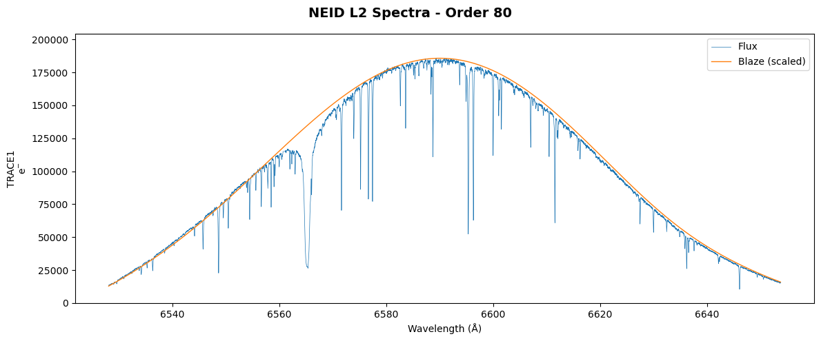
Plotting L2 Spectra
NEID has 3 traces in High Resolution mode (HR):
TRACE1: Science fiber
TRACE2: Calibration fiber (etalon)
TRACE3: Sky fiber
Let’s plot one order from the science traces.
[7]:
# Plot a single order from the three science traces
order = 80  # Choose an order to plot

fig, ax = plt.subplots(1, 1, figsize=(12, 5), sharex=True)
trace_num = 1
wave = l2[f'TRACE{trace_num}_WAVE'].data[order]
flux = l2[f'TRACE{trace_num}_FLUX'].data[order]
blaze = l2[f'TRACE{trace_num}_BLAZE'].data[order]

# Scale blaze for visualization
blaze_scaled = blaze * (np.nanmax(flux) / np.nanmax(blaze))

ax.plot(wave, flux, color='tab:blue', linestyle='-', lw=0.5, label='Flux')
ax.plot(wave, blaze_scaled, color='tab:orange', linestyle='-', lw=1, label='Blaze (scaled)')
ax.set_ylabel(f'TRACE{trace_num}'+'\ne$^{-}$')
ax.legend(loc='upper right')
ax.set_ylim(0, np.nanmax(flux) * 1.1)

ax.set_xlabel('Wavelength (\u212B)')
fig.suptitle(f'NEID L2 Spectra - Order {order}', fontsize=14, fontweight='bold')
plt.tight_layout()
plt.show()
Level 3: Stitched 1D Spectrum
Level 3 data contains a stitched 1D spectrum on a common wavelength grid with constant velocity spacing. The stitching process:
Divides out the blaze function
Resamples each order onto a common wavelength grid
Combines overlapping regions using inverse-variance weighting
Creating L3 from L2
L3 is created from an RVData-standard L2 file.
[8]:
# Create L3 from the standard L2 file
neid_l2 = RV2.from_fits(l2_standard_file)
neid_l3 = RV3()
neid_l3.convert_level2_to_level3(neid_l2)
# Save to FITS file
l3_standard_file = neid_l3.to_fits()
print(f"Created {l3_standard_file}")
Created neid_SL3_20231010T020006.fits
Using L3 Data
Reading the L3 File
[9]:
# Open the L3 file
l3 = fits.open(l3_standard_file)

# List extensions
print("L3 Extensions:")
for hdu in l3:
    print(f"  {hdu.name}")
L3 Extensions:
  PRIMARY
  INSTRUMENT_HEADER
  RECEIPT
  DRP_CONFIG
  EXT_DESCRIPT
  ORDER_TABLE
  STITCHED_CORR_SCI_FLUX
  STITCHED_CORR_SCI_WAVE
  STITCHED_CORR_SCI_VAR
Understanding L3 Extensions
For NEID with one science fiber, the stitched spectrum is stored are in STITCHED_CORR_SCI_* extensions:
STITCHED_CORR_SCI_WAVE/FLUX/VAR: Science fiber
[10]:
# Check which STITCHED extensions are present
stitched_exts = [hdu.name for hdu in l3 if 'STITCHED' in hdu.name]
print("Stitched spectrum extensions:")
for ext in stitched_exts:
    print(f"  {ext}")
Stitched spectrum extensions:
  STITCHED_CORR_SCI_FLUX
  STITCHED_CORR_SCI_WAVE
  STITCHED_CORR_SCI_VAR
Plotting the Stitched Spectrum
[11]:
# Plot the stitched spectrum for one trace
wave_ext = "STITCHED_CORR_SCI_WAVE"
flux_ext = "STITCHED_CORR_SCI_FLUX"
wave_l3 = l3[wave_ext].data
flux_l3 = l3[flux_ext].data

fig, ax = plt.subplots(figsize=(14, 5))
ax.plot(wave_l3, flux_l3, color='tab:blue', linestyle='-', lw=0.3, alpha=0.8)
ax.set_xlabel('Wavelength (\u212B)', fontsize=12)
ax.set_ylabel('Flux (e$^{-}$)', fontsize=12)
ax.set_title(f'NEID L3 Stitched Spectrum - Science Trace', fontsize=14, fontweight='bold')

# Zoom inset
ax.set_xlim(wave_l3[np.isfinite(wave_l3)].min(), wave_l3[np.isfinite(wave_l3)].max())
plt.tight_layout()
plt.show()

print(f"\nWavelength range: {np.nanmin(wave_l3):.1f} - {np.nanmax(wave_l3):.1f} Angstroms")
print(f"Number of pixels: {len(wave_l3)}")
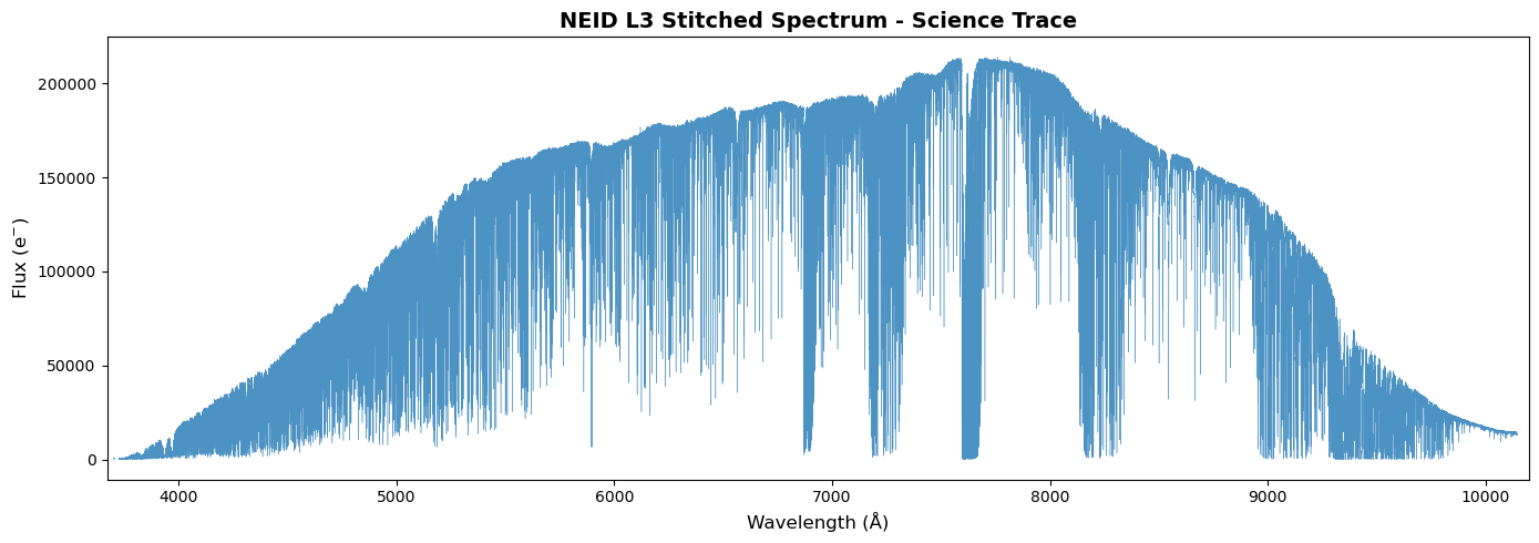
Wavelength range: 3670.0 - 10200.0 Angstroms
Number of pixels: 493473
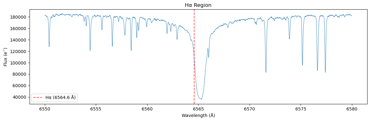
Zoomed View of Spectral Features
[12]:
# Zoom in on H-alpha region
if wave_ext in [hdu.name for hdu in l3]:
    fig, ax = plt.subplots(figsize=(12, 4))

    # H-alpha region
    mask = (wave_l3 > 6550) & (wave_l3 < 6580)
    ax.plot(wave_l3[mask], flux_l3[mask], color='tab:blue', linestyle='-', lw=0.7)
    ax.axvline(6564.6, color='red', ls='--', alpha=0.7, label='H\u03B1 (6564.6 \u212B)')
    ax.set_xlabel('Wavelength (\u212B)')
    ax.set_ylabel('Flux (e$^{-}$)')
    ax.set_title('H\u03B1 Region', fontsize=12)
    ax.legend()
    plt.tight_layout()
    plt.show()
Level 4: Radial Velocity Measurements
Level 4 data contains radial velocity (RV) measurements derived from the spectra. These can include:
Per-order RVs
Combined RV with uncertainty
Activity indicators
Creating L4 from Native NEID L2
L4 is typically created from native pipeline outputs that contain RV measurements. For NEID, the native L2 file includes CCF-derived RVs.
[13]:
# Create L4 from native NEID L2 file (which contains RV measurements)
neid_l4 = RV4.from_fits(native_l2_file, instrument="NEID")

# Save to FITS file
l4_standard_file = neid_l4.to_fits()
print(f"Created {l4_standard_file}")
Created neid_SL4_20231010T020006.fits
Using L4 Data
Reading the L4 File
[14]:
# Open the L4 file
l4 = fits.open(l4_standard_file)

# Examine primary header for RV info
hdr4 = l4[0].header
print(f"Object: {hdr4['OBJECT']}")
print(f"Observation time (BJD): {hdr4.get('BJDTDB', 'N/A')}")

# List extensions
print("\nL4 Extensions:")
for hdu in l4:
    print(f"  {hdu.name}")
Object: HD 185144
Observation time (BJD): 2460227.586673037

L4 Extensions:
  PRIMARY
  INSTRUMENT_HEADER
  RECEIPT
  DRP_CONFIG
  EXT_DESCRIPT
  RV1
  CCF1
  DIAGNOSTICS1
Examining the RV Table
The RV_TABLE extension contains the radial velocity measurements.
[15]:
# Check if RV_TABLE exists
if 'RV_TABLE' in [hdu.name for hdu in l4]:
    rv_table = Table(l4, hdu='RV_TABLE')
    print("RV Table columns:")
    print(rv_table.columns.tolist())
    print("\nRV Table:")
    print(rv_table)
else:
    print("RV_TABLE not found in this L4 file.")
    print("\nAvailable extensions:")
    for hdu in l4:
        if hdu.data is not None:
            print(f"  {hdu.name}: {type(hdu.data)}")
RV_TABLE not found in this L4 file.

Available extensions:
  INSTRUMENT_HEADER: <class 'numpy.ndarray'>
  RECEIPT: <class 'astropy.io.fits.fitsrec.FITS_rec'>
  DRP_CONFIG: <class 'astropy.io.fits.fitsrec.FITS_rec'>
  EXT_DESCRIPT: <class 'astropy.io.fits.fitsrec.FITS_rec'>
  RV1: <class 'astropy.io.fits.fitsrec.FITS_rec'>
  CCF1: <class 'numpy.ndarray'>
  DIAGNOSTICS1: <class 'astropy.io.fits.fitsrec.FITS_rec'>
Per-Order RVs
L4 files may also contain per-order RV measurements in the ORDER_RV extension.
[16]:
# Check for per-order RVs
if 'ORDER_RV' in [hdu.name for hdu in l4]:
    order_rv = l4['ORDER_RV'].data

    fig, ax = plt.subplots(figsize=(10, 5))
    orders = np.arange(len(order_rv))
    ax.scatter(orders, order_rv, s=20, alpha=0.7)
    ax.axhline(np.nanmedian(order_rv), color='red', ls='--', label=f'Median: {np.nanmedian(order_rv):.2f} m/s')
    ax.set_xlabel('Order Index')
    ax.set_ylabel('RV (m/s)')
    ax.set_title('Per-Order Radial Velocities')
    ax.legend()
    plt.tight_layout()
    plt.show()
else:
    print("ORDER_RV extension not found.")
ORDER_RV extension not found.
Summary
This tutorial demonstrated how to:
Create L2 from native NEID L2 file using
RV2.from_fits()Use L2 data: access headers, examine extensions, plot spectra
Create L3 from standard L2 using
neid_l2 = RV2.from_fits()andRV3().convert_level2_to_level3(neid_l2)Use L3 data: access stitched spectra, examine spectral features
Create L4 from native NEID L2 using
RV4.from_fits()Use L4 data: access RV measurements and per-order RVs
The standardized data format allows consistent access patterns across all EPRV instruments!
[17]:
# Clean up - close FITS files
l2.close()
l3.close()
l4.close()